Computer Science: March 2011

Tuesday, March 29, 2011

Different output for different compiler - C and C++

http://stackoverflow.com/questions/5467576/different-output-for-different-compiler-c-and-c

Some small and quick look at the various programs that could be possible.

Monday, March 21, 2011

OpenGL - My Scratch pad of programs

Program 1:

Monday, March 7, 2011

OpenGL and Physics - Some Learnings

MIT link
http://web.mit.edu/8.02t/www/802TEAL3D/visualizations/resources/resources.htm

Magnet Formulae:
http://www.netdenizen.com/emagnet/index.htm

Useful Links:

http://nehe.gamedev.net/data/lessons/lesson.asp?lesson=26

http://nehe.gamedev.net/data/lessons/lesson.asp?lesson=39

OpenGL Book:
Field visualization techniques..
http://books.google.co.in/books?id=rmgXE9jWjVgC&pg=PA561&lpg=PA561&dq=arrow+plot+in+openGL&source=bl&ots=UFEFAZpgvQ&sig=ysyP-wzNzLnXM3qEtfh6EX0V1us&hl=en&ei=A0eETfqSKYH0vQOzqNm8CA&sa=X&oi=book_result&ct=result&resnum=4&ved=0CDUQ6AEwAw#v=onepage&q&f=false

http://books.google.co.in/books?id=ZFrlULckWdAC&pg=PA290&lpg=PA290&dq=%22openGL+%22+solenoid+OR+%22bar+magnet%22+OR+%22vector+field%22&source=bl&ots=4AuJNUP6VX&sig=lzwLsqrVR7GR0vTBSIlU7GDLTxc&hl=en&ei=-VqETYelMYrsvQPhr-ndCA&sa=X&oi=book_result&ct=result&resnum=55&ved=0CIwDEOgBMDY#v=onepage&q=%22openGL%20%22%20solenoid%20OR%20%22bar%20magnet%22%20OR%20%22vector%20field%22&f=false

Good ppt:
http://www.authorstream.com/Presentation/Sophia-27431-25-Modeling-Simulating-Electromagnetism-Begin-Solution-Why-gravity-so-weak-Outlin-as-Entertainment-ppt-powerpoint/

GameDev:
http://www.gamedev.net/topic/541552-magnetic-fields-in-2d-space/
http://www.gamedev.net/topic/550586-magnetic-moment-of-a-moving-charge/
http://www.gamedev.net/topic/496159-circular-particle-system-optimization/
http://www.gamedev.net/topic/549373-calculating-the-angle-between-2-points-in-a-2d-system/

Image Based Flow Visualization: (The code works; Understand the code using the pdf file)
http://www.win.tue.nl/~vanwijk/ibfv/

http://www.devmaster.net/forums/showthread.php?t=13566

http://www.evilmadscientist.com/article.php/fields/print

Geometry using Matlab

Following are few of the Matlab interpreter commands to understand the geometries of some selected functions. These help me understand few of the complex convex optimization problems.

S.No.	Topic	Command	Description	Output
1	Norms	norm([3,4],1)	7	7
		norm([3,4],inf)	4	4
		norm([3,4],2) = norm([3,4])	5	5
2	2D plots	x=[-10:1:10]; plot(x, x.^2);	y = x^2
		x=[-10:1:10]; plot(x, 3.^x);	y = 3^x
		x=[-10:1:10]; plot(x, x.^3);	y = x^3
3	3D plots	t=[0:pi/30:6pi]; x=t.cos(t); y=t.*sin(t); z=t; plot3(x,y,z); grid on	x=t x cos(t) y=t x sin(t) z=t
		[x,y]=meshgrid(-2:1:2,-2:1:2); surf(x,y,x.^2-y.^2)	z =x²−y²
		[x,y]=meshgrid(-2:1:2,-2:1:2); surf(x,y,x.^2+y.^2)	z =x²+y²
		[x,y]=meshgrid(-2:0.1:2,-2:0.1:2); surf(x,y,x.^2-y.^2)	z =x²−y²
		[x,y]=meshgrid(-2:0.1:2,-2:0.1:2); surf(x,y,x.^2+y.^2)	z =x²+y²
		[x,y]=meshgrid(-2:0.1:2,-2:0.1:2); surfc(x,y,x.^2+y.^2)	z =x²+y²
4	Comparing graphs	[x,y]=meshgrid(-1:.1:1,-1:.1:1); subplot(1,2,1) surf(x,y,x.^2+y.^2) axis square subplot(1,2,2) contourf(x,y,x.^2+y.^2) axis square	z =x²+y²
		[x,y]=meshgrid(-1:.1:1,-1:.1:1); subplot(1,2,1) surf(x,y,sqrt(x.^2+y.^2) ) axis square subplot(1,2,2) contourf(x,y, sqrt(x.^2+y.^2) ) axis square
		[x,y]=meshgrid(-1:.1:1,-1:.1:1); subplot(1,2,1) surf(x,y,nthroot(x.^4+y.^4, 4)) axis square subplot(1,2,2) contourf(x,y,nthroot(x.^4+y.^4, 4))

References:

Friday, March 4, 2011

Using Apache's log4j library - how to?

Download the jar file from http://logging.apache.org/log4j/1.2/download.html.
Include it in the classpath by referencing it in the project as shown below..

Create a properties file "log4j.properties" (same as this file name) with following contents.

Write a simple class like this..

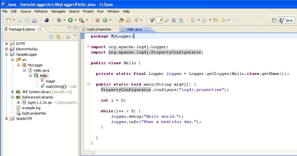
Wherever you create a new class just add the static member "logger" to your class, and start using it.

Start writing the log statements.

Collect all your log statements in your log file (as well as the console because of stdout in the properties file).

Thats it!! Enjoy debugging complex interleaving scenarios between multiple threads. You can use Notepad++ for filtering and using such log files when they are too big to browse through.